Chapter 3 Data import and processing
The SeaVal package provides some tools for data import and export. Currently it allows to read and write netcdf-files.
For reading and writing csv-files, see the data table functions fread and fwrite.
Data files are usually much smaller in netcdf format, which is also more flexible and more common, so this should be the preferred option.
3.1 Reading and writing netcdfs
The central function for importing netcdf-data as data.table is called netcdf_to_dt. It takes a filename of a netcdf (including directory path) as argument.
The example files we consider are hosted on ICPACs ftp server at SharedData/gcm/seasonal/202102.
data_dir = "example_data" # the directory the data is stored in, you need to adjust this to your platform.
fn = "CorrelationSkillRain_Feb-Apr_Feb2021.nc"
dt = netcdf_to_dt(file.path(data_dir, fn))
## File example_data/CorrelationSkillRain_Feb-Apr_Feb2021.nc (NC_FORMAT_CLASSIC):
##
## 1 variables (excluding dimension variables):
## float corr[lon,lat]
## lead: 0
## average_op_ncl: dim_avg_n over dimension(s): model
## type: 0
## time: 13
## _FillValue: -9999
##
## 3 dimensions:
## time Size:0 *** is unlimited *** (no dimvar)
## lat Size:77
## units: degrees_north
## lon Size:66
## units: degrees_east
##
## 6 global attributes:
## units: mm
## MonInit_month: 2
## valid_time: Feb-Apr
## creation_date: Mon Feb 15 06:59:57 EAT 2021
## Conventions: None
## title: Correlation between Cross-Validated and Observed Rainfallprint(dt)## lon lat corr
## <num> <num> <num>
## 1: 20.5 -11.5 -0.4893801
## 2: 21.0 -11.5 -0.3525713
## 3: 21.5 -11.5 -0.3583783
## 4: 22.0 -11.5 -0.4319133
## 5: 22.5 -11.5 -0.4062470
## ---
## 2277: 49.5 22.5 -0.3988679
## 2278: 50.0 22.5 -0.2976854
## 2279: 50.5 22.5 -0.3071221
## 2280: 51.0 22.5 -0.1081869
## 2281: 51.5 22.5 0.1165779The function requires the file name including directory path. You can specify the path relative to you work directory (which you can see by running getwd() and change by setwd). The easiest approach is to set your work directory to the directory the netcdf is located in. Be aware that directory separators differ between Linux, Mac and Windows, but you can use the function file.path to avoid issues.
By default, the function prints out all the information it gets from the netcdf, including units, array sizes etc.
This can be turned off by the verbose argument of the function: setting it to 0 suppresses all messages, setting it to 1 only prints units of the variables.
The default value is 2.
A netcdf-file always contains variables (such as precip or temperature) and dimension variables (such as longitude or time). The function netcdf_to_dt by default tries to extract all variables into a single data table that also contains all dimension variables that are indexing at least one variable: For example, the netcdf file above has three dimension variables: lon,lat, and time (which is empty). It has one variable (‘corr’) that is indexed by lon and lat, therefore the resulting data table has three columns: corr, lon and lat.
It is possible to have netcdfs with several variables, which may moreover be indexed by different dimension variables.
In this setting, the default behavior of reading all variables and cramming them into a single data table may be inappropriate.
Say, for example, we have a netcdf with three dimension variables lon, lat and time, and it has a variable precipitation[lon,lat,time] and a second variable grid_point_index[lon,lat]. The resulting data table would have the columns lon, lat, time, precipitation, and grid_point_index.
This is not very memory efficient because the grid_point_indices are repeated for every instance of time.
Moreover, in this case we probably don’t need the grid_point_index anyway.
We can use the vars argument of the netcdf_to_dt function to extract only selected variables. So, in this example, netcdf_to_dt('example_file.nc', vars = 'precipitation') would do the trick.
Merging the data tables for all variables is particularly expensive in memory when you have multiple variables that have different dimension variables. For large netcdfs with many variables and many dimension variables this can easily get out of hand. In this case you can use netcdf_to_dt('example_file.nc',trymerge = FALSE).
This will return a list of data tables, one data table for each variable, containing only the variable values and its dimension variables.
If you have two or more variables that do not share a dimension variable, the function requires you to set trymerge = FALSE.
For the example above, the resulting data table looks like this:
ggplot_dt(dt,
          mn = 'Corr. skill rain Feb-Apr, Feb initialized', # title
          rr = c(-1,1), # range of the colorbar
          discrete_cs = TRUE,binwidth = 0.4) # discretize colorbar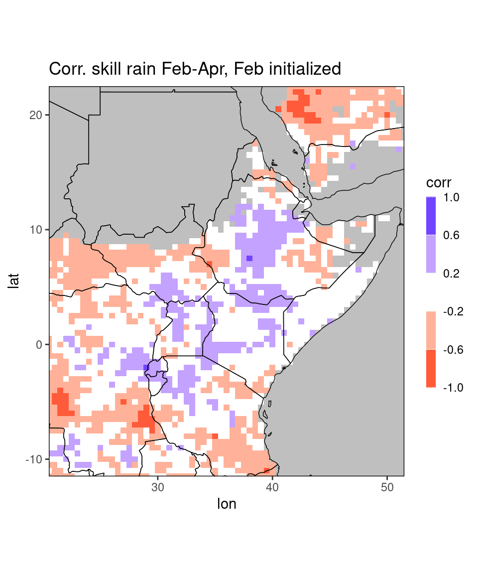
fn = "CorrelationSkillRain_Mar-May_Feb2021.nc"

dt = netcdf_to_dt(file.path(data_dir, fn), verbose = 0)

ggplot_dt(dt[!is.na(corr)], # here we suppress missing values
          mn = 'Corr. skill rain Mar-May, Feb initialized', # title
          rr = c(-1,1), # range of the colorbar
          discrete_cs = TRUE, binwidth = 0.4) # discretize colorbar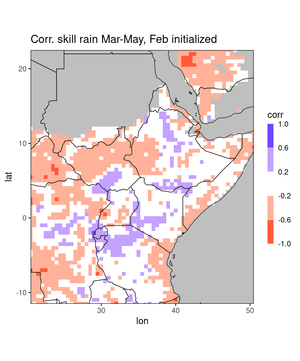
Especially for large netcdfs it is much faster to just load parts of the data. The netcdf_to_dt-function allows this kind of subsetting, see function documentation for details.
An example for loading only parts of the correlation data looks like this:
fn = "CorrelationSkillRain_Feb-Apr_Feb2021.nc"
dt = netcdf_to_dt(file.path(data_dir, fn),verbose = 0,
                  subset_list = list(lon = c(25,35), lat = c(0,10)))

ggplot_dt(dt)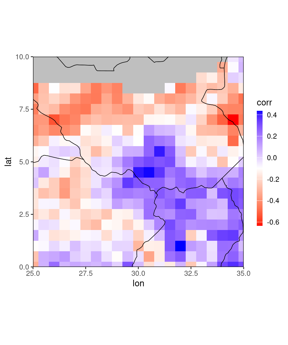
Similarly, for writing netcdf files from data tables, the package has a function dt_to_netcdf. The function requires a data table as input and a file name as output. Based on the column names of your data tale, it will try to guess which columns contain dimension variables and which value variables and ask for confirmation. If you don’t provide units, the function will prompt you for it. See ?dt_to_netcdf for more details.
3.2 Downloading and processing CHIRPS data
Evaluation of forecasts always requires observations to assess the forecast performance. Moreover, usually we are interested whether the prediction was as good or better than a naive climatological forecast. This requires establishing a climatology which requires access to past observations as well. To this end, the SeaVal package provides code that simplifies the download and use of the CHIRPS monthly means rainfall data set. The CHIRPS data is created by the Climate Hazard Group of UC Santa Barbara. The data is mirrored on the IRI data library, which allows downloading (area-)subsetted data.
While for some netcdfs it is possible to read them directly online, this is not possible from the IRI data library. Also, then your access to the data depends on the speed of your internet connection. To avoid this the SeaVal package provides functions for downloading and processing CHIRPS data.
The CHIRPS data is on the very high spatial resolution of 0.05 degree lon/lat. While this makes for great-looking plots, it also means that the entire CHIRPS data is roughly 800 MB on disk, even though it is just monthly means. If you do not have that much disk space to spare, the download function has a resolution-argument that allows you to upscale the data to 0.5 degree lon/lat during downloading. The default is to download high-resolution but also upscale, since the much smaller upscaled version is easier to work with.
The different options are:
resolution = 'both': This is the default and downloads the original data and additionally derives an upscaled version that is easier to work with. This is recommended when you have a bit over 800 MB of disk space to spare.resolution = 'low': Downloads the file and upscales it before saving. Only the coarse resolution is kept. In this format, the entire data is roughly 8 MB on disk.resolution = 'high': Downloads only the original data, and does not upscale. You need roughly 800 MB. This is not recommended and barely has any benefits overboth.
In order to download all available CHIRPS monthly mean data to your local machine, it is sufficient to run the function
download_chirps_monthly()The first time you run this function, it will ask you to specify a data directory on your local machine. This path is saved and from now on generally used by the SeaVal-package for storing and loading data. You can later look up which data directory you specified by running data_dir(). In theory, you should not change your data directory. If, for some reason, you need to change this, you can run data_dir(set_dir = TRUE). However, this simply generates a new empty data directory and specifies the new directory as lookup path for the SeaVal package. It does not move over or delete data in the old data directory - you have to do that manually.
The download_chirps_monthly function comes with several useful options. You can specify months and years you want to download (the default is to download everything there is). Moreover, the function automatically looks up which months have been downloaded previously and only loads the data for months that you are still missing. If you want to re-download and overwrite existing files, you can set update = FALSE.
By default, the function downloads only data for the greater-horn-of-Africa area. You can change this setting to download larger datasets such as Africa or even global, see function documentation, but be aware of long download times and disk storage.
After having downloaded the CHIRPS data, you can load it using the function load_chirps:
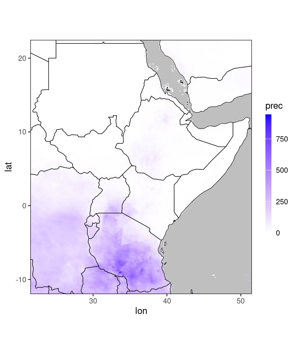
dt = load_chirps()## Starting 06/2024, load_chirps() returns rainfall in mm (or mm/month), no longer in mm/day. Monthly chirps uses 30-day calendar so in order to convert to mm/day you can simply divide by 30.print(dt)## lon lat prec year month
## <num> <num> <num> <num> <num>
## 1: 22.0 -12.0 209.4447632 1981 1
## 2: 22.5 -12.0 219.0442810 1981 1
## 3: 23.0 -12.0 270.9567261 1981 1
## 4: 23.5 -12.0 272.3134460 1981 1
## 5: 24.0 -12.0 261.1191406 1981 1
## ---
## 1796794: 49.5 22.5 0.2549688 2023 9
## 1796795: 50.0 22.5 0.2447293 2023 9
## 1796796: 50.5 22.5 0.2382571 2023 9
## 1796797: 51.0 22.5 0.2176941 2023 9
## 1796798: 51.5 22.5 0.1917573 2023 9# example plot
pp = ggplot_dt(dt[year == 2022 & month == 1], high = 'blue', midpoint = 0)
plot(pp)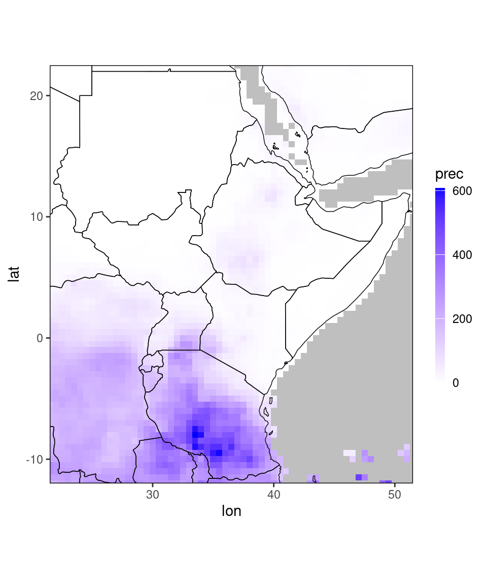
By default, the upscaled data is loaded (which is smaller in memory and loads faster) if it is available. Moreover, the function provides options to only load subsets of the data, and to load the data in the original high resolution (if you downloaded the high resolution):
dt = load_chirps(years = 2022, months = 1, resolution = 'high')## Starting 06/2024, load_chirps() returns rainfall in mm (or mm/month), no longer in mm/day. Monthly chirps uses 30-day calendar so in order to convert to mm/day you can simply divide by 30.print(dt)## lon lat prec year month
## <num> <num> <num> <num> <num>
## 1: 21.50 22.475 0.3189361 2022 1
## 2: 21.55 22.475 0.3187493 2022 1
## 3: 21.60 22.475 0.3183813 2022 1
## 4: 21.65 22.475 0.3179317 2022 1
## 5: 21.70 22.475 0.1653149 2022 1
## ---
## 327774: 40.60 -11.975 167.4485931 2022 1
## 327775: 49.15 -11.975 245.7680817 2022 1
## 327776: 49.20 -11.975 533.7239380 2022 1
## 327777: 49.25 -11.975 469.3838501 2022 1
## 327778: 49.30 -11.975 487.2277222 2022 1# example plot
ggplot_dt(dt)