Chapter 4 Utilities
SeaVal does help you to calculate evaluation metrics, once you have your data in the right format.
The package is focussing on evaluating tercile forecasts. Such forecasts issue three probabilities: for a below normal, a normal, and an above normal category, which are defined from the local and seasonal climatology terciles.
For evaluation, SeaVal expects your data to look something like this:
## Key: <lat, lon, month, year>
##          lat   lon month  year below normal above terc_cat
##        <num> <num> <int> <int> <num>  <num> <num>    <int>
##     1: -11.5  35.0    11  2018  0.16   0.28  0.56        0
##     2: -11.5  35.0    11  2019  0.12   0.36  0.52        0
##     3: -11.5  35.0    11  2020  0.44   0.40  0.16       -1
##     4: -11.5  35.0    12  2018  0.16   0.36  0.48        0
##     5: -11.5  35.0    12  2019  0.12   0.40  0.48        1
##    ---
## 12404:  23.0  35.5    11  2019  0.24   0.44  0.32        1
## 12405:  23.0  35.5    11  2020  0.36   0.40  0.24        0
## 12406:  23.0  35.5    12  2018  0.20   0.40  0.40        0
## 12407:  23.0  35.5    12  2019  0.40   0.40  0.20        0
## 12408:  23.0  35.5    12  2020  0.40   0.28  0.32       -1
Specifically, we have a data table with some dimension variables (lat, lon, month, year). For each coordinate (each unique combination of values of dimension variables) we have three predicted probabilities (below, normal, above) and a
corresponding outcome/observation (terc_cat). We follow the conventions that probabilities are given between 0 and 1 (not in percent), and represent below-normal observations as -1, normal as 0 and above normal as 1. If we manage to get our forecasts and observations into this format, SeaVal can derive a large variety of evaluation metrics automatically. For example, we can get reliability diagrams from the data table above like this:
rel_diag(dt)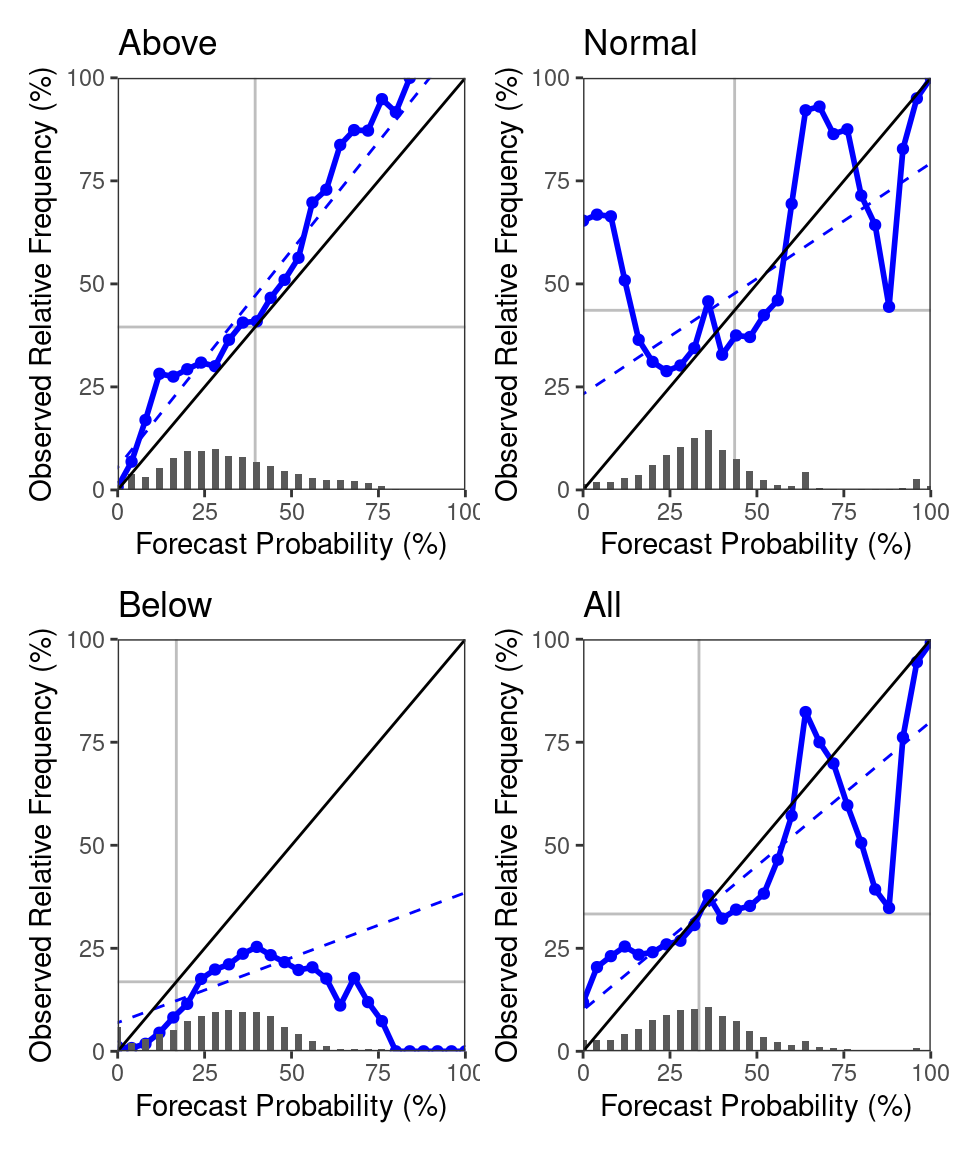
Of course, your data will originally not look exactly as the data table above, so we have to get it into this format first.
In fact, when you use SeaVal, this becomes your main task for forecast evaluation. Once you have the data in this format, you can lean back and use all the various evaluation functions provided by SeaVal discussed in the next chapter.
4.1 Getting your data into the right format
In this chapter, we will look at a variety of utility-functions provided by SeaVal that help you to get your data into this format. The first challenge is often that you have an ensemble forecast and need to derive a tercile forecast from it. After reading in ensemble forecast data with netcdf_to_dt, it will usually look something like this example dataset:
dt = copy(ecmwf_monthly)
dt[,c('below', 'normal', 'above') := NULL] # example data contains tercile probabilities, but these will usually not be included if you just loaded some forecast
print(dt)
## Index: <month>
## lon lat year month prec member
## <num> <num> <int> <int> <num> <int>
## 1: 22 13.0 2018 11 0.00 1
## 2: 22 13.0 2018 11 0.00 2
## 3: 22 13.0 2018 11 2.58 3
## 4: 22 13.0 2018 12 0.00 1
## 5: 22 13.0 2018 12 0.00 2
## ---
## 37220: 51 11.5 2020 11 79.20 2
## 37221: 51 11.5 2020 11 7.35 3
## 37222: 51 11.5 2020 12 25.23 1
## 37223: 51 11.5 2020 12 23.16 2
## 37224: 51 11.5 2020 12 44.07 3If we want to derive tercile probabilities for this, we can derive the climatology-terciles from the forecast climatology. Then, for each year, we can count how many ensemble members fall into which tercile and use this for predicting tercile probabilities. For example, say for a given gridpoint and month, the first climatology tercile is 1.5 mm and the second is 5.5 mm. That means that a third of all ensemble members (from all years) that predict precipitation for this location and month predicted precipitation below 1.5 mm, and another third predicted above 5.5 mm. Now, for a give year, say 80% of all members predict above 5.5 mm, and 20% predict between 1.5 mm and 5.5 mm. This would correspond to a probability forecast of 0 for below normal, 0.2 for normal and 0.8 for above normal.
SeaVal has a single function that does all of these calculations for you. The function is called tfc_from_efc (tercile forecast from ensemble forecast). Let’s have a look:
tfc_from_efc(dt)## lat lon month year below normal above
## <num> <num> <int> <int> <num> <num> <num>
## 1: 13.0 22 11 2018 0.6666667 0.0000000 0.3333333
## 2: 13.0 22 12 2018 0.0000000 1.0000000 0.0000000
## 3: 13.0 22 11 2019 1.0000000 0.0000000 0.0000000
## 4: 13.0 22 12 2019 0.3333333 0.6666667 0.0000000
## 5: 13.0 22 11 2020 0.3333333 0.0000000 0.6666667
## ---
## 12404: 11.5 51 12 2018 0.3333333 0.3333333 0.3333333
## 12405: 11.5 51 11 2019 0.3333333 0.3333333 0.3333333
## 12406: 11.5 51 12 2019 0.3333333 0.3333333 0.3333333
## 12407: 11.5 51 11 2020 0.6666667 0.3333333 0.0000000
## 12408: 11.5 51 12 2020 0.3333333 0.3333333 0.3333333We can see that the tercile probabilities are always thirds (meaning, they are 0, 0.333, 0.667 or 1). This is because the original data table contains only a three-member forecast. Note that the original data table only contains years 2018-2020, so the forecast climatology is based on only three years. So this forecast is likely not very good. It is, therefore, important to include fore- and hindcast in the data table before you run tfc_from_efc, because the function establishes the forecast terciles from the data, and a larger number of years (typically around 30) is required to get reliable climatology terciles. By default, the function tries to guess which column contains the ensemble forecasts (see fc_cols()). If you use a column name that is not recognized, you can provide it as the f-argument, so tfc_from_efc(dt,f = 'prec') would have worked, too.
When you have turned your forecasts into tercile forecasts, you typically still have to combine them with observations. To this end we can use the function combine. Let us combine the forecasts above with the monthly CHIRPS example data:
forecasts = tfc_from_efc(dt)
dt = combine(forecasts, chirps_monthly)
print(dt)
## Key: <lat, lon, month, year>
## lat lon month year below normal above prec terc_cat
## <num> <num> <int> <int> <num> <num> <num> <num> <int>
## 1: -11.5 35.0 11 2018 0.0000000 0.6666667 0.3333333 33.99 0
## 2: -11.5 35.0 11 2019 0.0000000 0.3333333 0.6666667 62.07 0
## 3: -11.5 35.0 11 2020 1.0000000 0.0000000 0.0000000 29.07 -1
## 4: -11.5 35.0 12 2018 0.0000000 0.3333333 0.6666667 205.74 0
## 5: -11.5 35.0 12 2019 0.6666667 0.0000000 0.3333333 342.57 1
## ---
## 12404: 23.0 35.5 11 2019 0.3333333 0.3333333 0.3333333 11.37 1
## 12405: 23.0 35.5 11 2020 0.3333333 0.3333333 0.3333333 7.20 0
## 12406: 23.0 35.5 12 2018 0.3333333 0.3333333 0.3333333 3.96 0
## 12407: 23.0 35.5 12 2019 0.3333333 0.6666667 0.0000000 3.75 0
## 12408: 23.0 35.5 12 2020 0.3333333 0.0000000 0.6666667 3.24 -1This data table is now in the format we need it in, and we can begin evaluation. Note that the combine-function returns a warning if the data tables you are combining have columns with the same names that are not recognized as dimension variables.
A typical example is if both your forecasts and observations contain a column called precipitation or similar. In this case, you should rename one of these columns using the data.table-function setnames.
For other functions for combining data tables have a look at the functions merge, cbind, and rbindlist from the data.table-package.
In this example, we were a bit lucky that the observations already contained a column terc_cat. If they don’t, we can add such a column using the add_tercile_cat-function. This function will add the tercile category for each observation relative to local climatology. The terciles for local climatology are established directly from the data, so your data table should contain multiple years of observations, ideally something like 30.
4.2 Converting monthly to seasonal data
The example datasets chirps_monthly and ecmwf_monthly contain monthly values. If we want to work with seasonal data instead, we can use the convert_monthly_to_seasonal() function.
By default, the function considers the seasons MAM (March - May), JJAS (June - August) and OND (October - December), since these are the standard target seasons for the GHACOFs, see Section Plots for the Greater Horn of Africa.
However, you can also specify other seasons by the consecutive letters of their starting months, e.g. 'MAMJ' for March-April-May-June, or 'DJ' for December-January.
Both example datasets only consider data for November and December, so here we work with the season ND:
print(chirps_monthly)## lon lat prec month year terc_cat
## <num> <num> <num> <int> <int> <int>
## 1: 22.0 -12.0 199.68 11 1991 1
## 2: 22.0 -11.5 198.87 11 1991 1
## 3: 22.0 -11.0 157.86 11 1991 0
## 4: 22.0 -10.5 144.15 11 1991 -1
## 5: 22.0 -10.0 153.96 11 1991 -1
## ---
## 209036: 51.5 21.0 7.20 12 2020 -1
## 209037: 51.5 21.5 6.54 12 2020 -1
## 209038: 51.5 22.0 6.15 12 2020 -1
## 209039: 51.5 22.5 4.86 12 2020 -1
## 209040: 51.5 23.0 4.17 12 2020 -1chirps_seasonal = convert_monthly_to_seasonal(chirps_monthly, seasons = "ND")## Warning in convert_monthly_to_seasonal(chirps_monthly, seasons = "ND"): The data contains tercile categories.
## I cannot derive seasonal tercile categories from monthly ones.
## Please derive tercile categories AFTER converting to seasonal values.## The data in the following columns is aggregated:
## precprint(chirps_seasonal)## lat lon year prec season
## <num> <num> <int> <num> <char>
## 1: -12.0 22.0 1991 434.07 ND
## 2: -11.5 22.0 1991 457.02 ND
## 3: -11.0 22.0 1991 433.02 ND
## 4: -10.5 22.0 1991 375.12 ND
## 5: -10.0 22.0 1991 413.67 ND
## ---
## 104516: 21.0 51.5 2020 7.20 ND
## 104517: 21.5 51.5 2020 8.01 ND
## 104518: 22.0 51.5 2020 9.27 ND
## 104519: 22.5 51.5 2020 7.41 ND
## 104520: 23.0 51.5 2020 5.64 NDNote that the derived dataset contains no longer a month column, but a season column instead. The function printed out a warning telling us that it cannot derive tercile categories for the ND season from tercile categories for each month. Indeed, if for example November was below normal and December was above normal, the season total could be either below normal, normal or above normal. The outcome depends on the total amounts for the months, but also the historical values during the climatological period.
Similarly, we cannot derive tercile predictions for a season from tercile predictions for each month. Therefore, the rule of thumb is to first aggregate to season, and only afterwards calculate tercile probabilities and categories.
For the derived dataset chirps_seasonal, the obs column contains the sum of obs-values over all months in the season.
This is appropriate for precipitation, as considered here, but for surface temperature the mean should be calculated. This can be changed in the function arguments, see ?convert_monthly_to_seasonal.
You can also control the grouping behaviour:
Here, the sum is calculated separately for all lat, lon, and year (or grouped by lat, lon, and year). This is exactly what we want and in most cases the function can guess how you want to aggregate.
However, if it guesses wrongly, you can control grouping behavior and which columns to aggregate by changing the function parameters.
4.3 Upscaling
It is quite common to get forecasts and observations on different lon/lat grids. In this context, the best solution for evaluation is to upscale them to a common grid. E.g., if one of the two datasets is on finer resolution, you could upscale this dataset to the coarser grid of the other dataset. SeaVal can do this for you, as long as both grids are regular longitude/latitude grids. The function to do this is called
upscale_regular_lon_lat. It uses conservative interpolation, which is equivalent to bilinear interpolation if both grids are of the same spatial resolution (and are just shifted against each other).
However, conservative interpolation works better than bilinear interpolation for upscaling data from a finer to a coarser grid.
Let us look at an example:
dt = copy(chirps_monthly)
ggplot_dt(dt)
## Warning in modify_dt_map_plotting(dt = dt, data_col = data_col): The data table contains multiple levels per lon/lat. The following selection is plotted:
## month = 11
## year = 1991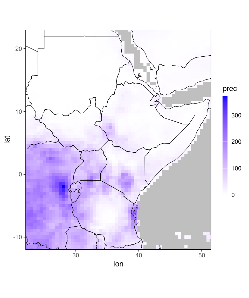
# get coarser grid as data table, in this case full-degree lon/lats
coarse_grid = as.data.table(expand.grid(lon = -180:180, lat = -90:90))
print(coarse_grid)
## lon lat
## <int> <int>
## 1: -180 -90
## 2: -179 -90
## 3: -178 -90
## 4: -177 -90
## 5: -176 -90
## ---
## 65337: 176 90
## 65338: 177 90
## 65339: 178 90
## 65340: 179 90
## 65341: 180 90dt_us = upscale_regular_lon_lat(dt, coarse_grid,
uscols = 'prec') #specify the column you want to upscale
ggplot_dt(dt_us)## Warning in modify_dt_map_plotting(dt = dt, data_col = data_col): The data table contains multiple levels per lon/lat. The following selection is plotted:
## month = 11
## year = 1991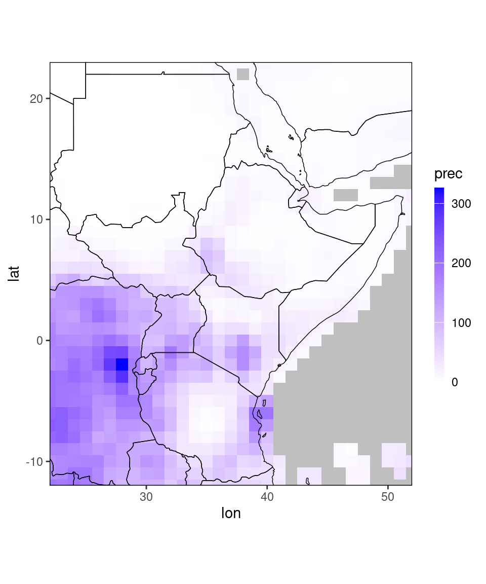
4.4 Other utilities
There are a few more functions contained in SeaVal that are frequently useful. We will not go too much into detail here, but provide a list of the functions. See the function documentations for more details:
add_climatology: Adds a climatology column to a data table with observations or forecasts.add_country: Adds a column with the country name to a data table that contains lon/lat coordinates.add_tercile_probs: Adds tercile probabilities to a data table with ensemble forecast values.MSD_to_YMFrequently, months are given in the format ‘Months since 1960-01-01’ (or some other origin date). This function converts time given in this ‘Months since date’ format into the usual year/month format.restrict_to_countryRestricts a data table to the gridpoints in a specific country.restrict_to_GHARestricts a data table to the gridpoints falling into the Greater Horn of Africa region.