Chapter 1 Getting Started
1.1 Installation
Just like any other package, you can install the SeaVal-package from CRAN, the Comprehensive R Archive Network. In order to do this, simply open R and type
install.packages('SeaVal')This installs the SeaVal package including all dependencies.
After installation, you can load SeaVal by typing
library(SeaVal)## Loading required package: data.table## Loading required package: ggplot2The rest of the tutorial is organized as follows. We will first give a few examples how to use Rs data table syntax to perform typical tasks required for evaluation. Thereafter, we will show how SeaVal can be used to visualize data as spatial maps. This will be followed by examples how to import forecasts and download observations data. Thereafter, the tutorial shows how observations and predictions can be combined into a suitable dataset for evaluation. Finally, it shows how to evaluate different types of forecasts
1.2 examples of data.table syntax
Here, we show some examples of basic operations on data tables.
A short but comprehensive introduction to data.tables syntax can be found here.
The SeaVal package comes with two example data sets for highlighting functionality. The first one contains monthly mean precipitation over the GHA region for the OND season provided by CHIRPS:
library(data.table)
data("chirps_monthly")
print(chirps_monthly)
## lon lat prec month year terc_cat
## <num> <num> <num> <int> <int> <int>
## 1: 22.0 -12.0 199.68 11 1991 1
## 2: 22.0 -11.5 198.87 11 1991 1
## 3: 22.0 -11.0 157.86 11 1991 0
## 4: 22.0 -10.5 144.15 11 1991 -1
## 5: 22.0 -10.0 153.96 11 1991 -1
## ---
## 209036: 51.5 21.0 7.20 12 2020 -1
## 209037: 51.5 21.5 6.54 12 2020 -1
## 209038: 51.5 22.0 6.15 12 2020 -1
## 209039: 51.5 22.5 4.86 12 2020 -1
## 209040: 51.5 23.0 4.17 12 2020 -1A short description of the dataset is also provided:
?chirps_monthlychirps_monthly is a data table, which is an enhanced data frame. Most operations available for data frames can typically be directly applied to data tables. The data table package moreover provides simplified notation for fundamental operations, such as subsetting, performing calculations on columns and aggregation or grouping for calculations. Examples for subsetting are
chirps_monthly[month == 11] # extract the data for November
chirps_monthly[year %between% c(1995,1999)] # extract the data for 1995 - 1999
chirps_monthly[1000:2000] # extract rows 1000 - 2000
chirps_monthly[month == 11][lon > 30][terc_cat == 0] #chained subsetting: get all November values at locations with longitude >30 that had normal rainfall (terc_cat == 0)
chirps_monthly[month == 11 & lon > 30 & terc_cat == 0] # different syntax, same effect.
We can subset either by row indices (third example) or by logical expressions (all other examples). Subsetting always returns a data table, e.g. chirps_monthly[1] returns a one-row data table containing the first row of chirps_monthly.
Next, let’s look at examples for operations on columns:
chirps_monthly[,mean(prec)] # get the mean precipitation (over all locations, months, years)## [1] 56.38002chirps_monthly[,mean_prec := mean(prec)] # create a new column in the data table containing the mean
chirps_monthly[,prec := 30*prec] # transform precipitation from unit mm/day to mm (per month)
print(chirps_monthly)## lon lat prec month year terc_cat mean_prec
## <num> <num> <num> <int> <int> <int> <num>
## 1: 22.0 -12.0 5990.4 11 1991 1 56.38002
## 2: 22.0 -11.5 5966.1 11 1991 1 56.38002
## 3: 22.0 -11.0 4735.8 11 1991 0 56.38002
## 4: 22.0 -10.5 4324.5 11 1991 -1 56.38002
## 5: 22.0 -10.0 4618.8 11 1991 -1 56.38002
## ---
## 209036: 51.5 21.0 216.0 12 2020 -1 56.38002
## 209037: 51.5 21.5 196.2 12 2020 -1 56.38002
## 209038: 51.5 22.0 184.5 12 2020 -1 56.38002
## 209039: 51.5 22.5 145.8 12 2020 -1 56.38002
## 209040: 51.5 23.0 125.1 12 2020 -1 56.38002Note in all cases the ‘,’ after ‘[’ which tells data table that you’re doing an operation rather than trying to subset.
More generally, data.table-syntax follows the logic dt[(subsetting),(computing),(grouping)], so by putting one comma we indicate that we want to compute.
Grouping is another important operation we will learn about later.
We can also put things together and subset and compute simultaneously. In this case, the subsetting is specified first, followed by a comma followed by the operation:
chirps_monthly[month == 11 , mean(prec)] # get the mean precipitation for November (over all locations, years)## [1] 1709.858(Note that the mean is much larger now because we changed units…). Finally, we can perform operations over aggregated groups:
dt_new = chirps_monthly[, mean(prec), by = .(lon,lat,month)]
print(dt_new)
## lon lat month V1
## <num> <num> <int> <num>
## 1: 22.0 -12.0 11 4737.60
## 2: 22.0 -11.5 11 4883.43
## 3: 22.0 -11.0 11 4950.93
## 4: 22.0 -10.5 11 5078.55
## 5: 22.0 -10.0 11 5500.29
## ---
## 6964: 51.5 21.0 12 229.08
## 6965: 51.5 21.5 12 217.74
## 6966: 51.5 22.0 12 193.77
## 6967: 51.5 22.5 12 165.09
## 6968: 51.5 23.0 12 146.70Here, the ‘by’ command (after the second comma) tells data table to perform the calculation (mean) for each unique instance of lon, lat, and month separately. As a result, the mean is taken only over all years, and a separate mean is derived for each location and each month. Therefore, this operation derives the monthly local climatology. As we can see, the output is a data table containing all columns in by and a column named V1 containing the output of the operation. That’s a bit impractical, so let’s rename the last column:
setnames(dt_new,'V1','clim') # take the data table from above and rename column 'V1' into 'clim'It’s also possible to name the column directly while dt_new is created, like this:
dt_new = chirps_monthly[,.(clim = mean(prec)),by = .(lon,lat,month)]
# same as above, but with simultaneously setting the name of the new column
The .() notation is a data.table-abbreviation for list(), see the official data table introduction for more details.
We can now also combine grouping, calculating and subsetting:
dt_new = chirps_monthly[year %in% 1995:2000, .(clim = mean(prec)), by = .(lon,lat,month)]
# computes climatology based on the years 1995-2000 only.
In the examples above we create a new data table containing the climatology. If we instead want to add the climatology as a new column to chirps_monthly directly, we need to use the := operator:
chirps_monthly[,clim := mean(prec), by = .(lon,lat,month)] # add the climatology column directly into chirps_monthly.This showcases some of the functionalities and syntax of the data.table package. There’s a lot more to it and it is strongly recommended having a look at
this introduction to data.table if you are not familiar with data tables.
Since data tables are the native data format of SeaVal, a good understanding of how to manipulate data tables will make your life much easier.
We’ll finish this section by an example where we compute the MSE for raw ecmwf forecasts, combining all the operations we’ve seen above:
data("chirps_monthly") # reload data to reverse the changes made in the examples above.
data("ecmwf_monthly") # get example hindcasts from ecmwf

print(ecmwf_monthly)
## Index: <month>
## lon lat year month prec member below normal above
## <num> <num> <int> <int> <num> <int> <num> <num> <num>
## 1: 22 13.0 2018 11 0.00 1 0.80 0.04 0.16
## 2: 22 13.0 2018 11 0.00 2 0.80 0.04 0.16
## 3: 22 13.0 2018 11 2.58 3 0.80 0.04 0.16
## 4: 22 13.0 2018 12 0.00 1 0.00 1.00 0.00
## 5: 22 13.0 2018 12 0.00 2 0.00 1.00 0.00
## ---
## 37220: 51 11.5 2020 11 79.20 2 0.32 0.40 0.28
## 37221: 51 11.5 2020 11 7.35 3 0.32 0.40 0.28
## 37222: 51 11.5 2020 12 25.23 1 0.36 0.28 0.36
## 37223: 51 11.5 2020 12 23.16 2 0.36 0.28 0.36
## 37224: 51 11.5 2020 12 44.07 3 0.36 0.28 0.36# merge observations and predictions into a single data table:
setnames(chirps_monthly,'prec','obs')
# rename the 'prec' column in the observation data table to 'obs',
# in order to avoid name clashes, since ecmwf_monthly also contains a column 'prec',
# containing the predictions for precip.
dt = combine(ecmwf_monthly,chirps_monthly)
# combine the two data tables.
print(dt)## Key: <lat, lon, month, year>
## lat lon month year prec member below normal above obs terc_cat
## <num> <num> <int> <int> <num> <int> <num> <num> <num> <num> <int>
## 1: -11.5 35.0 11 2018 93.15 1 0.16 0.28 0.56 33.99 0
## 2: -11.5 35.0 11 2018 67.68 2 0.16 0.28 0.56 33.99 0
## 3: -11.5 35.0 11 2018 168.42 3 0.16 0.28 0.56 33.99 0
## 4: -11.5 35.0 11 2019 128.88 1 0.12 0.36 0.52 62.07 0
## 5: -11.5 35.0 11 2019 78.63 2 0.12 0.36 0.52 62.07 0
## ---
## 37220: 23.0 35.5 12 2019 3.81 2 0.40 0.40 0.20 3.75 0
## 37221: 23.0 35.5 12 2019 1.56 3 0.40 0.40 0.20 3.75 0
## 37222: 23.0 35.5 12 2020 4.59 1 0.40 0.28 0.32 3.24 -1
## 37223: 23.0 35.5 12 2020 5.91 2 0.40 0.28 0.32 3.24 -1
## 37224: 23.0 35.5 12 2020 0.30 3 0.40 0.28 0.32 3.24 -1dt[,ens_mean := mean(prec),by = .(lon,lat,year,month)]
# get the ensemble mean as a new column.
# The mean is here grouped over all dimension variables excluding 'member',
# therefore the ensemble mean is returned. In other words, a separate mean
# is calculated for every instance of lon, lat, year and month.
mse_dt = dt[,.(mse = mean((obs - ens_mean)^2)), by = .(lon,lat,month)] # create a new data.table containing the mse by location and month
print(mse_dt)## lon lat month mse
## <num> <num> <int> <num>
## 1: 35.0 -11.5 11 2844.2605333
## 2: 35.0 -11.5 12 4714.4014667
## 3: 35.5 -11.5 11 3951.7420000
## 4: 35.5 -11.5 12 5182.9996333
## 5: 36.5 -11.5 11 4107.8679000
## ---
## 4132: 35.5 22.5 12 2.4708667
## 4133: 36.0 22.5 11 93.1384667
## 4134: 36.0 22.5 12 0.8163667
## 4135: 35.5 23.0 11 23.8516333
## 4136: 35.5 23.0 12 0.6400333# plot mse for October:
ggplot_dt(mse_dt[month == 11],'mse',midpoint = 0, rr = c(-50000,50000)) 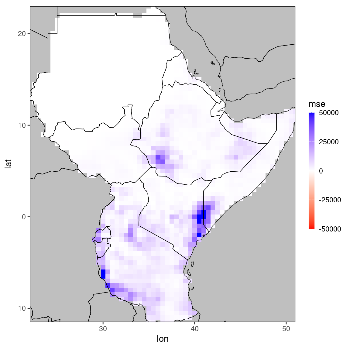
The function ggplot_dt is used to create spatial plots from data stored in data tables. The next section highlights how to use this function and how the generated plots can be manipulated.